Installing
You can install mpathwear from Github.
remotes::install_github("koenniem/mpathwear")Let’s load some libraries we will use for this vignette.
library(dplyr)
#>
#> Attaching package: 'dplyr'
#> The following objects are masked from 'package:stats':
#>
#>     filter, lag
#> The following objects are masked from 'package:base':
#>
#>     intersect, setdiff, setequal, union
library(mpathwear)
Overview
This vignette shows a minimal workflow for using the
mpathwear package. In this vignette, we will use the
example data included with the package. This example dataset was
downloaded directly from m-Path (see the manual
for how to download the data) and should thus be very similar to a
dataset from a real study.
First, we will set a path variable that points to the
data, in this case from within mpathwear:
# Path to the example data shipped with the package
path <- system.file("extdata", "example.csv", package = "mpathwear")
Next, we can use the read_mpathwear() function to read
the data into R.
Note that if you downloaded the data iteratively from m-Path
(e.g. every day to have backups), the data will overlap as the data
export in m-Path is cumulative. Nevertheless,
read_mpathwear() will automatically remove duplicate rows
but this will fail if a day was not yet completed.
# Read the data (this can also be a directory containing multiple exported CSVs)
raw <- read_mpathwear(path)

head(raw)
#> # A tibble: 3 × 9
#>   connectionId legacyCode  code     alias initials accountCode lastCreatedAtUnix
#>   <chr>        <chr>       <chr>    <chr> <chr>    <chr>                   <dbl>
#> 1 123456       !1234@abc12 !abcd e… exam… exa      abc12           1764164955448
#> 2 123456       !1234@abc12 !abcd e… exam… exa      abc12           1764165350362
#> 3 123456       !1234@abc12 !abcd e… exam… exa      abc12           1764166043493
#> # ℹ 2 more variables: dynamicData <list>, dailyData <list>
Cleaning the data
read_mpathwear() returns the raw exported rows
containing JSON-encoded daily and dynamic measurements. The functions
clean_daily_data() and clean_dynamic_data()
unpack these JSON blobs and return tidy tibbles suitable for plotting
and analysis.
# Clean interday (daily) summary data
# Drop the dynamicData column since this cannot be combined with daily data anyway
daily <- raw |>
  select(-"dynamicData") |>
  clean_daily_data()

glimpse(daily)
#> Rows: 387
#> Columns: 18
#> $ connectionId      <chr> "123456", "123456", "123456", "123456", "123456", "1…
#> $ legacyCode        <chr> "!1234@abc12", "!1234@abc12", "!1234@abc12", "!1234@…
#> $ code              <chr> "!abcd efgh", "!abcd efgh", "!abcd efgh", "!abcd efg…
#> $ alias             <chr> "example_user", "example_user", "example_user", "exa…
#> $ initials          <chr> "exa", "exa", "exa", "exa", "exa", "exa", "exa", "ex…
#> $ accountCode       <chr> "abc12", "abc12", "abc12", "abc12", "abc12", "abc12"…
#> $ lastCreatedAtUnix <dbl> 1.764165e+12, 1.764165e+12, 1.764165e+12, 1.764165e+…
#> $ day               <date> 2025-11-12, 2025-11-12, 2025-11-12, 2025-11-12, 202…
#> $ category          <chr> "Activity", "Activity", "Activity", "Activity", "Act…
#> $ subcategory       <chr> "Steps", "CoveredDistance", "FloorsClimbed", "Elevat…
#> $ variable          <chr> "Steps", "CoveredDistance", "FloorsClimbed", "Elevat…
#> $ value             <chr> "4402", "3661.0", "5", "15.0", "2370", "195", "14", …
#> $ timezoneOffset    <int> 60, 60, 60, 60, 60, 60, 60, 60, 60, 60, 60, 60, 60, …
#> $ generation        <chr> NA, NA, NA, "calculation", NA, NA, "calculation", NA…
#> $ created_at        <dttm> 2025-11-26 13:48:37, 2025-11-26 13:48:37, 2025-11-2…
#> $ data_source       <chr> "Garmin", "Garmin", "Garmin", "Garmin", "Garmin", "G…
#> $ description       <chr> "sum of steps (including the manually added values)"…
#> $ available_sources <list> <"Apple", "Beurer", "Decathlon", "Fitbit", "Garmin"…
For larger datasets, clean_dynamic_data() may take some
time to finish running (e.g. several) minutes.
# Clean intraday (dynamic) data
# Drop the dailyData column since this cannot be combined with dynamic data anyway
dynamic <- raw |>
  select(-"dailyData") |>
  clean_dynamic_data()

glimpse(dynamic)
#> Rows: 37,332
#> Columns: 19
#> $ connectionId      <chr> "123456", "123456", "123456", "123456", "123456", "1…
#> $ legacyCode        <chr> "!1234@abc12", "!1234@abc12", "!1234@abc12", "!1234@…
#> $ code              <chr> "!abcd efgh", "!abcd efgh", "!abcd efgh", "!abcd efg…
#> $ alias             <chr> "example_user", "example_user", "example_user", "exa…
#> $ initials          <chr> "exa", "exa", "exa", "exa", "exa", "exa", "exa", "ex…
#> $ accountCode       <chr> "abc12", "abc12", "abc12", "abc12", "abc12", "abc12"…
#> $ lastCreatedAtUnix <dbl> 1.764165e+12, 1.764165e+12, 1.764165e+12, 1.764165e+…
#> $ start_time        <dttm> 2025-11-23 11:36:00, 2025-11-12 09:11:15, 2025-11-2…
#> $ end_time          <dttm> 2025-11-23 11:39:00, 2025-11-12 09:12:15, 2025-11-2…
#> $ category          <chr> "Stress", "Cardiovascular", "Sleep", "Activity", "Ca…
#> $ subcategory       <chr> "Stress", "HeartRate", "SleepInBedDuration", "Steps"…
#> $ variable          <chr> "Stress", "HeartRate", "SleepInBedBinary", "Steps", …
#> $ value             <chr> "27", "82", "true", "14.0", "68", "54", "25", "true"…
#> $ tz_offset         <int> 60, 60, 60, 60, 60, 60, 60, 60, 60, 60, 60, 60, 60, …
#> $ generation        <chr> NA, NA, "automated_measurement", "automated_measurem…
#> $ created_at        <dttm> 2025-11-26 13:48:37, 2025-11-26 13:48:37, 2025-11-2…
#> $ data_source       <chr> "Garmin", "Garmin", "Garmin", "Garmin", "Garmin", "G…
#> $ description       <chr> "stress measured during that period scaling from 0 t…
#> $ available_sources <list> "Garmin", <"Apple", "Beurer", "Fitbit", "Garmin", "…
Example charts
Below are a few example charts that demonstrate common visualizations for wearable data. For an overview of all charting functions, see the reference section.
Coverage
First of all, we may want to know to what extent data was actually
gathered. We can inspect this using a coverage chart that plots whether
data was present or absent over time. For the daily data, we can use
daily_coverage_chart() that plots each participant ID on
the y-axis and day number (0 for day 1, 1 for
day 2 etc.) on the x-axis with variables displayed as facets. This gives
a good indication of how complete the data is.
Note that not necessarily all variables will be present for all days.
First of all, some devices may not support some variables which means
that they will always be absent. Second, some variables are not
continuous but rather event-driven. For instance, if there was no high
activity event on a certain day, the ActivityHighDuration
will be absent. In a way, this is an implicit 0 that you
may want to take into account when running analyses.
daily_coverage_chart(daily)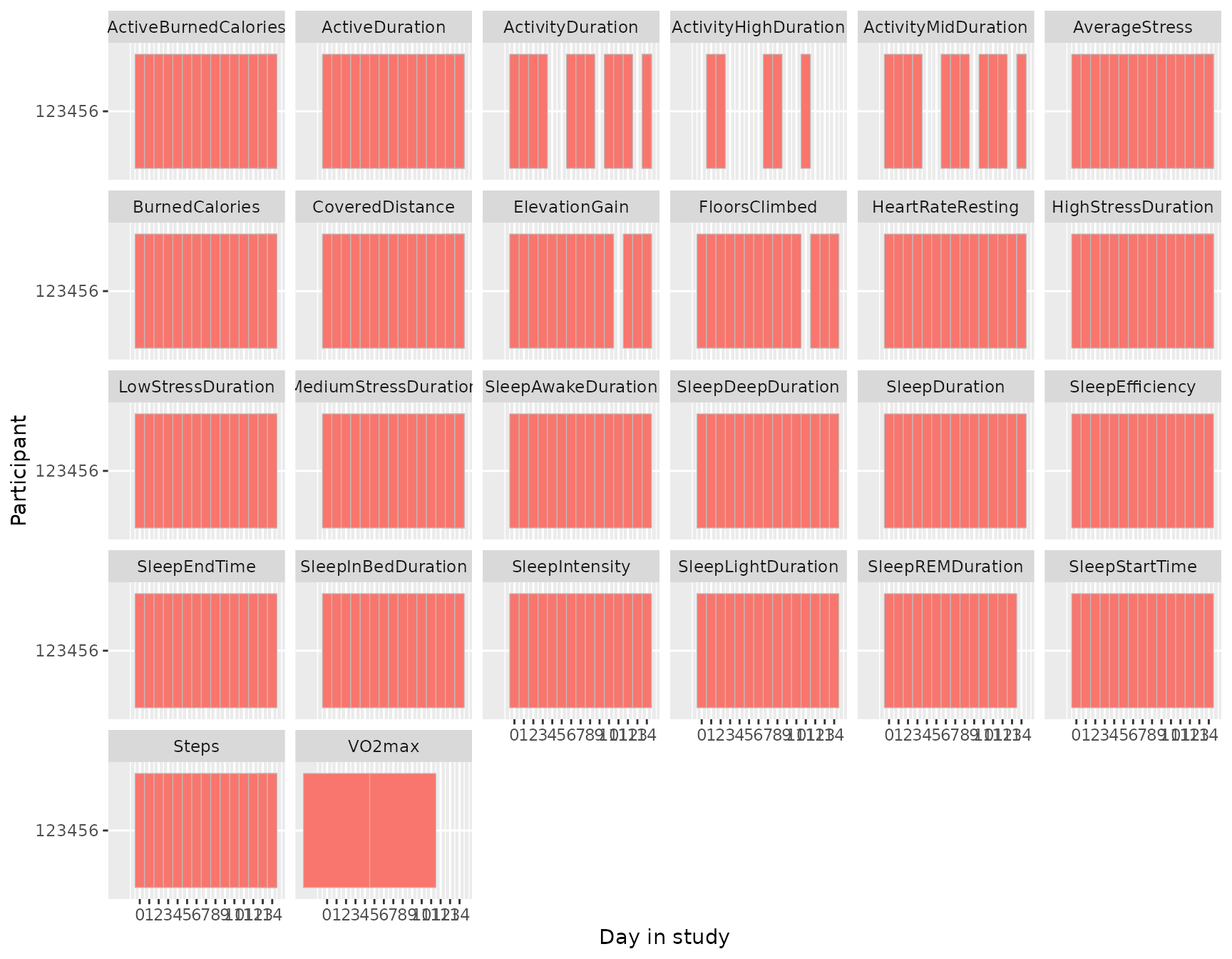
We can do the same thing for the intraday data using
coverage_chart(), only here are the bars not per day but
rather displayed by their actual duration. So, while the daily coverage
chart shows you whether data is present or not for that day, the
intradaily coverage chart shows exactly how often data is collected
across time spans.
Like the daily coverage chart, “missing” data does not need to be
truly missing. For instance, RunBinary does not occur if
the participant did not run during the recorded period. On the other
hand, one would hope that HeartRate is somewhat
continuously present. In conclusion, this chart shows you how often data
is present for each variable over time.
coverage_chart(dynamic)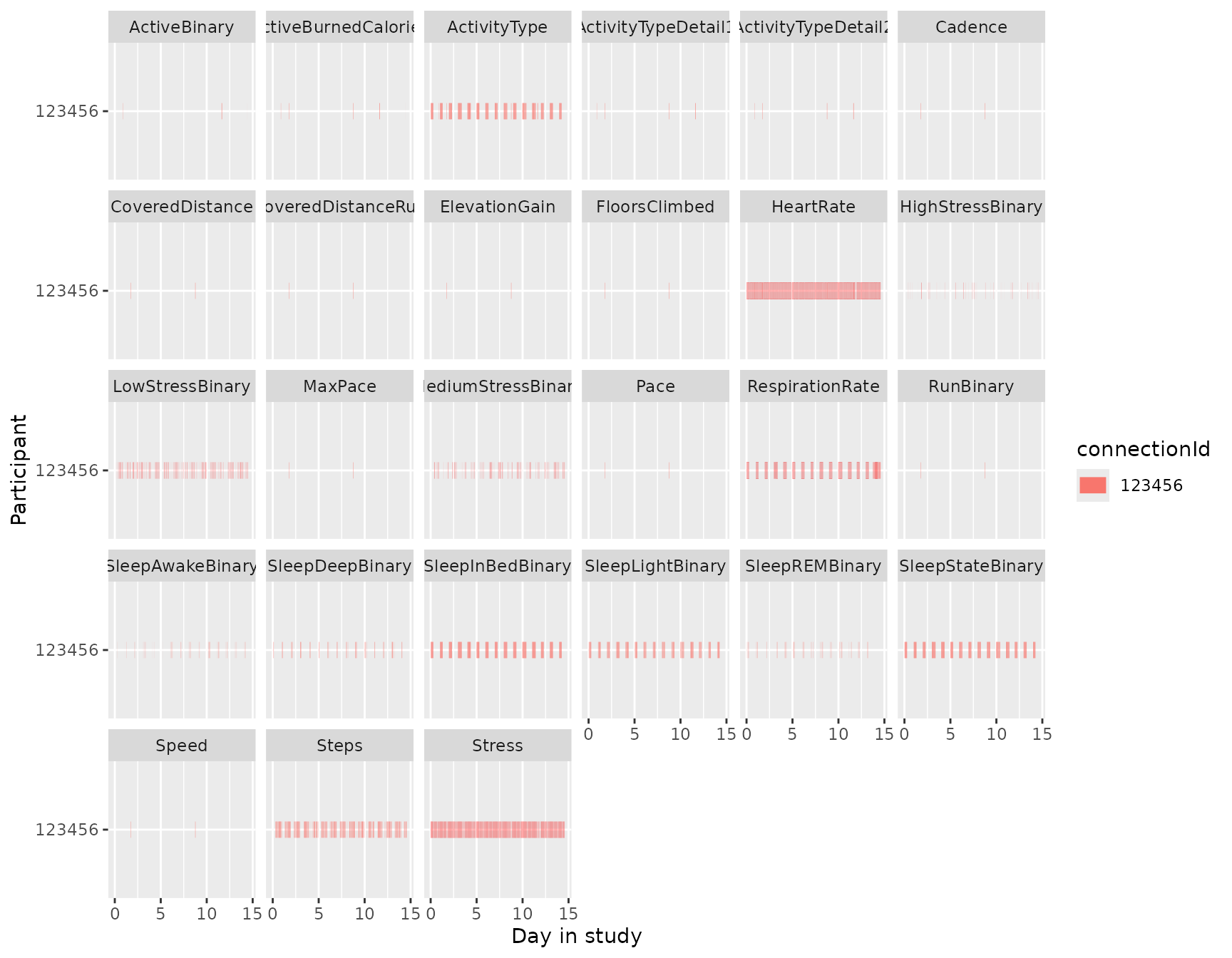
Daily summary chart
The daily_chart() function visualizes daily summary
variables over time for a single participant. Each variable is plotted
in its own facet.
daily_chart(daily)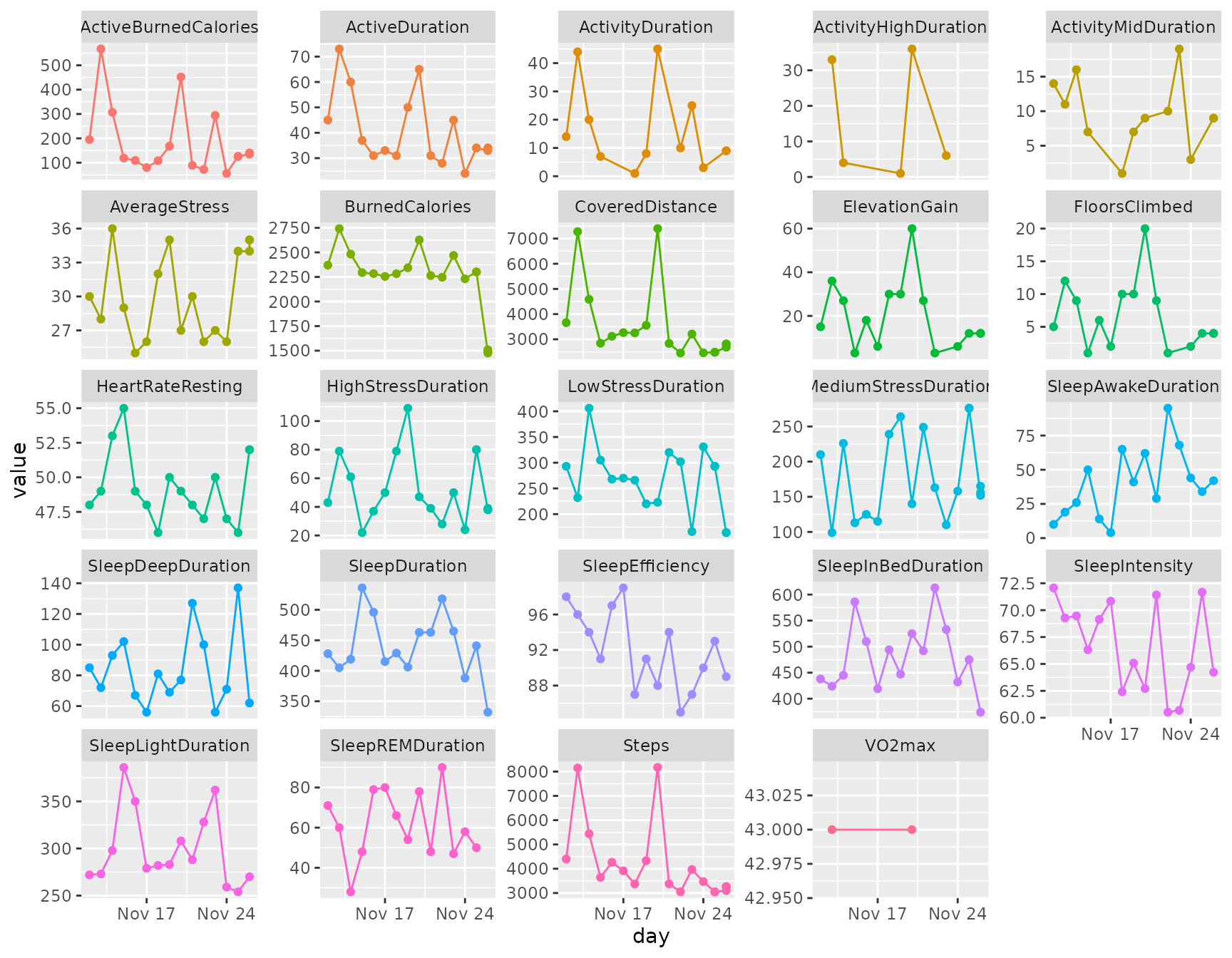
Heart rate
heart_rate_chart() shows the heart rate over time as
well as the average heart rate of that day.
heart_rate_chart(dynamic)
#> Warning: Removed 1 row containing missing values or values outside the scale range
#> (`geom_segment()`).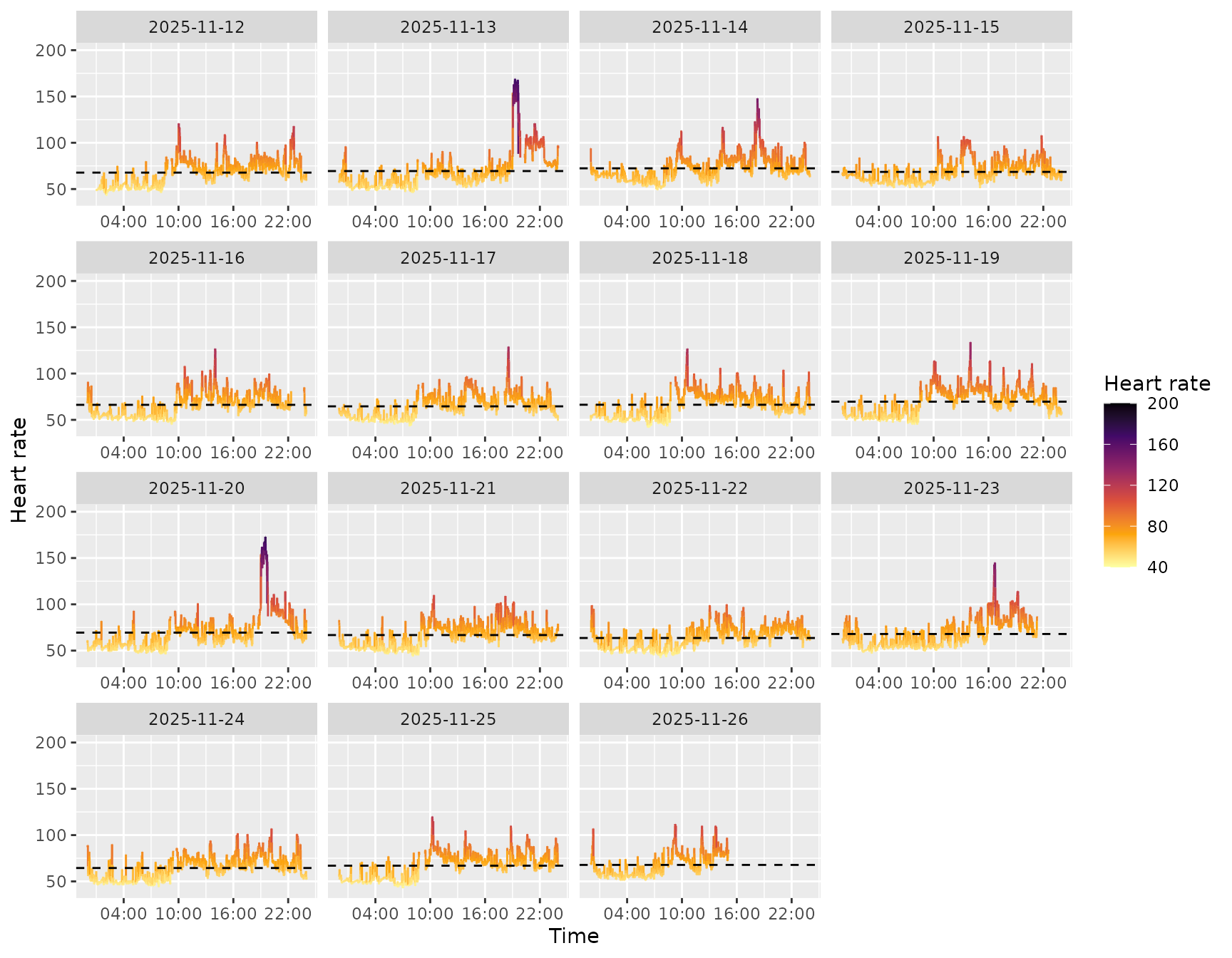
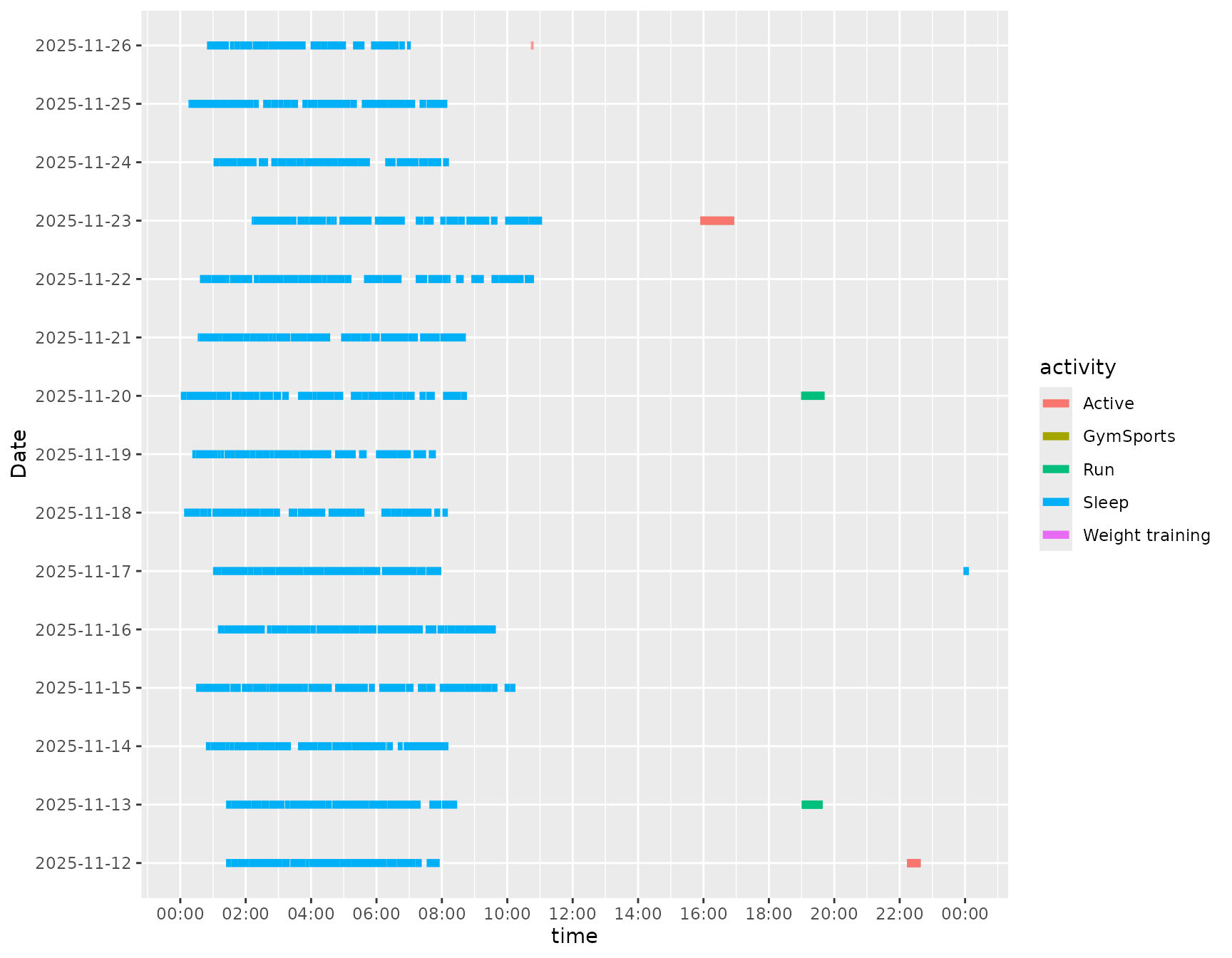
Sleep
The package includes helpers for sleep visualisation and commonly
used sleep metrics. The sleep_chart() function visualises
sleep stages (awake, REM, light, deep) across nights. The other helpers
compute durations and scores from intraday (dynamic) data.
sleep_chart(dynamic)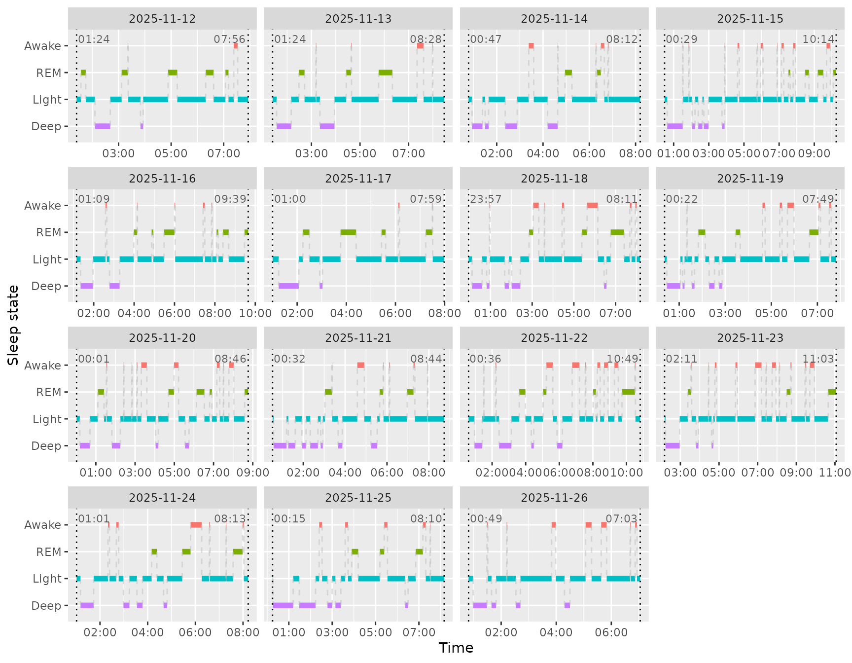
Below we show a few of the sleep metric helpers. Each returns a
tibble with day and the corresponding metric (in seconds
for intraday-derived metrics). To merge them, we can use
Reduce() to call each function and add them to the result
using full_join().
Reduce(
  \(x, y) full_join(x, y, by = "day"),
  list(
    sleep_duration(dynamic),
    sleep_deep_duration(dynamic),
    sleep_efficiency(dynamic)
  )
)
#> # A tibble: 15 × 4
#>    day        SleepDuration SleepDeepDuration SleepEfficiency
#>    <date>             <int>             <int>           <dbl>
#>  1 2025-11-12         23520              2460           0.974
#>  2 2025-11-13         25440              4320           0.955
#>  3 2025-11-14         26700              5580           0.942
#>  4 2025-11-15         35158              6120           0.915
#>  5 2025-11-16         30600              4020           0.973
#>  6 2025-11-17         25140              3360           0.990
#>  7 2025-11-18         29640              4860           0.868
#>  8 2025-11-19         26820              4140           0.908
#>  9 2025-11-20         31500              4620           0.882
#> 10 2025-11-21         29520              7620           0.941
#> 11 2025-11-22         36780              6000           0.845
#> 12 2025-11-23         31971              3360           0.872
#> 13 2025-11-24         25920              4260           0.898
#> 14 2025-11-25         28500              8220           0.928
#> 15 2025-11-26         22440              3720           0.888